1. bidirectional(양방향) RNN 이란 ?

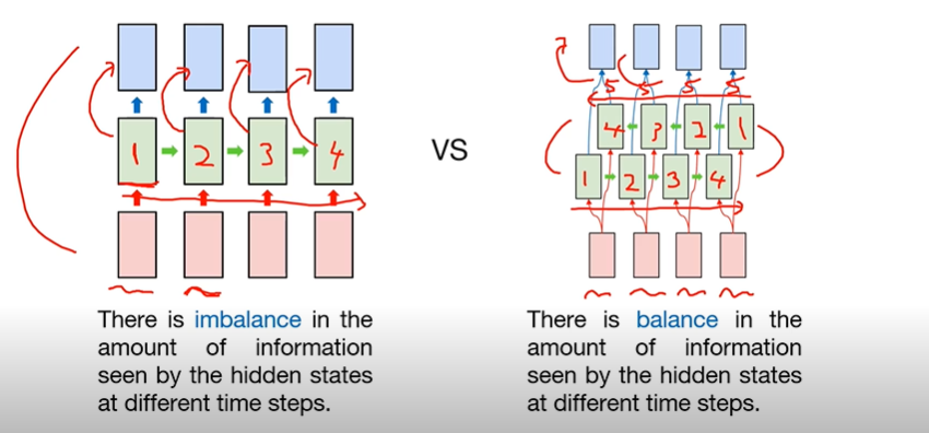
이전 강의까지는 모두 RNN을 모두 단방향으로만 활용을 하였는데, 사실 이 방식은 정보의 불균형이 존재한다. 풀어서 설명하자면 다음과 같다.
단방향 RNN이 시퀀스의 첫 번째 토큰을 읽었을 때, 첫 번째 토큰에 대한 hidden states에는 정보가 1만큼 저장되어 있다고 하면, 그 정보를 기반으로 첫 번째 아웃풋을 내고, 다시 RNN이 시퀀스의 두 번째 토큰을 읽었을 때는 첫 번째 토큰에 대한 hidden states의 정보도 활용하여 두 번째 아웃풋을 출력하고, 또 다시 RNN이 시퀀스의 세 번째 토큰을 읽었을 때는 첫 번째와 두 번째 토큰에 대한 hidden states의 정보를 활용하여 세 번째 아웃풋을 내는 방식이므로 정보의 불균형이 생길 수 밖에 없는 구조이다.
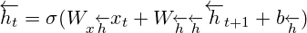
이러한 구조적 문제점을 해결하기 위해 등장한 것이 bidirectional RNN이다. bidirectional RNN은 2개의 Hidden Layer을 가지고 있다. 전방향 상태(Forward States)정보를 가지고 있는 hidden layer와 후방향 상태(Backward States) 정보를 가지고 있는 hidden layer가 있고, 이 둘은 서로 연결되어 있지 않은 구조로 형성되어 있다. 그러나 입력되는 토큰은 이 두 가지 hidden layer에 모두 전달되고 아웃풋 layer은 이 두 가지 hidden layer의 값을 모두 받아서 계산한다. 이를 수식으로 나타내면 아래와 같다.

...시간

...전방향(forward) hidden layer의 활성값(activation) output

...전방향(backward) hidden layer의 활성값(activation)

....output,output layer의 output

...sigmoid나 ReLU같은 활성 함수(activation function)
은 다음과 같이 계산하다.

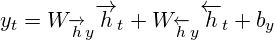
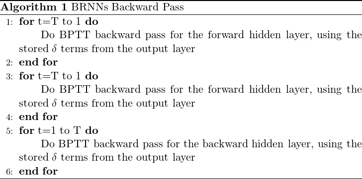
Forwardpass 계산을 진행하는 것을 일반적은 RNNs와 같다. 단지, Forward hidden layer와 Backward hidden layer에 input 값을반대 방향(opposite)으로 집어넣고, Output layer 값은 두방향의 Hidden layer에 모든 input이 적용된 후에 계산한다는 점이 차이점이다. 아래는 이 과정을 알고리즘 형태로 나타낸 것이다.
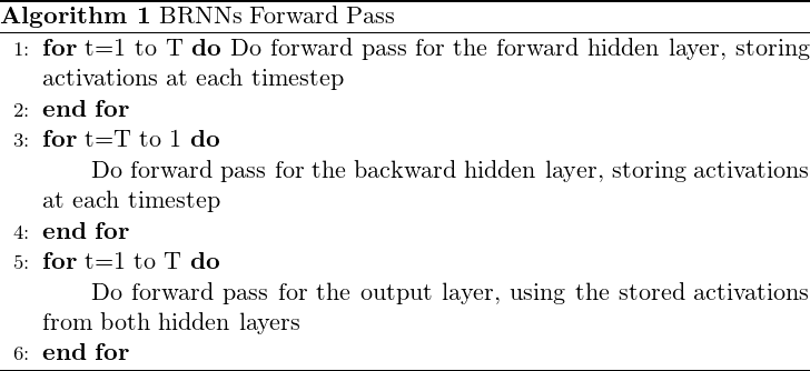
Backwardpass의 가중치를 업데이트 할때는, 기본적인 RNNs와 같이BPTT를 이용한다. 단지, output layer에서 모든 시간에 대해 에러값

를 먼저 계산하고, 이를 Forward hidden layer와 Backward hidden layer에반대 방향(opposite)으로 전달한다는 점이 차이점이다. 아래는 이 과정을 알고리즘 형태로 나타낸 것이다.
BPTT(Back propagation Throgh Time, 通時的誤差逆伝搬)란?
기존의 오차역전파(back propagation)는 시간을 고려하지 않고 그 때의 입력, 출력, 교사신호로만 모델을 수정하였지만,
BTPP는 여기에 과거의 시간을 고려해 수정을 한다. 시간 t의 hidden layer는 시간t의 입력 시간t-1의 hidden laye뿐만 아니라 시간 t-2이전의 hidden layer의 값에도 영향을 주기 때문에 좀 더 시간을 거슬러 올라가서 수정하자는 것이다.
계산식에 대해 알아보고 싶다면 아래의 두 링크를 참고바란다.
https://aikorea.org/blog/rnn-tutorial-3/
https://kiyukuta.github.io/2013/12/09/mlac2013_day9_recurrent_neural_network_language_model.html#back-propagation-through-time-bptt
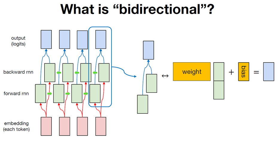
bidirectional RNN의 동작에 대해 조금 더 자세히 살펴보자. 어떠한 시퀀스를 tokenizaiton한 후, embedding layer를 활용하여 각각의 토큰을 numeric vector로 변환한다. (이전 예제들에서는 토큰을 one hot vector로 변환했었다.) 이렇게 변환된 토큰을 forward RNN과 backward RNN이 읽고, 각각의 RNN의 hidden states를 합친다. 정확히는 forward RNN의 hidden states와 backward RNN의 hidden states를 concatenate하는 방식으로 새로운 벡터를 생성하고 그 벡터를 weight와 bias를 활용하여 목적에 맞게 생성, 모델링하는 구조이다. 여기서 weight와 bias는 모든 토큰의 hidden states에 대해 동일하게 적용된다.
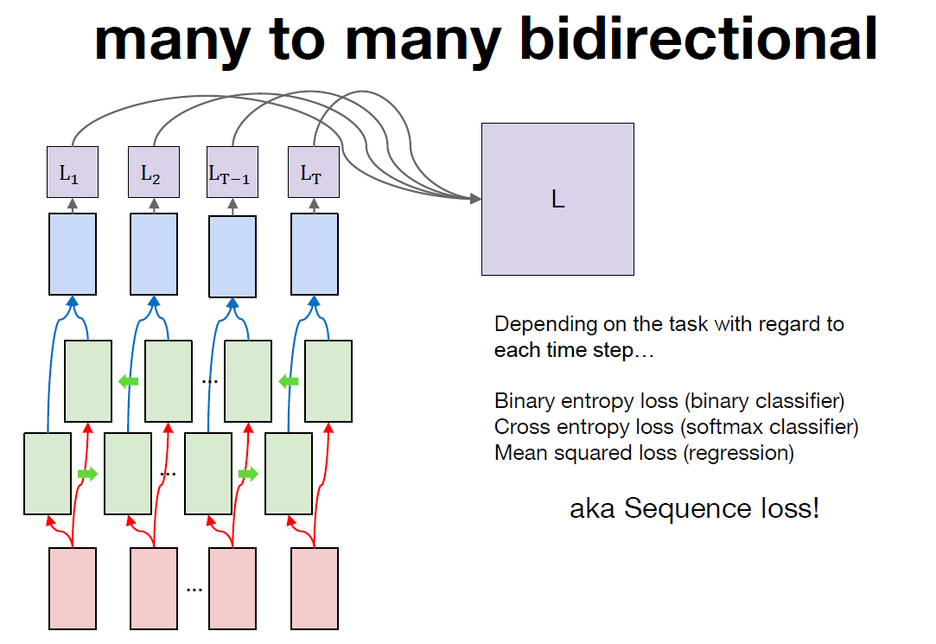
loss를 계산하는 방법은 이전 강의에서 RNN을 many to many방식과 동일하게 sequence loss를 계산한다. ( 각 토큰마다의 bidirectional RNN의 출력과 정답을 비교하여 loss를 계산하고 마스킹을 활용하여 데이터 간의 길이를 맞추기 위한 pad토큰을 제외한 실제 데이터에 유효한 토큰들에 대해서 loss를 계산하고 이를 판별한다. )이렇게 계산된 sequence loss로 bidirectional RNN을 back propagation을 통해서 학습할 수 있다.
2. bidirectional RNN 구현
이전과 거의 코드가 동일하나, RNN을 bidirectional로 구현한 부분만 다르다.
1) Importing libraries
# setup
import numpy as np
import tensorflow as tf
import matplotlib.pyplot as plt
from tensorflow import keras
from tensorflow.keras import layers
from tensorflow.keras import Sequential, Model
from tensorflow.keras.preprocessing.sequence import pad_sequences
from pprint import pprint
%matplotlib inline

print(tf.__version__)
2.1.0
2) Preparing dataset
# example data
sentences = [['I', 'feel', 'hungry'],
     ['tensorflow', 'is', 'very', 'difficult'],
     ['tensorflow', 'is', 'a', 'framework', 'for', 'deep', 'learning'],
     ['tensorflow', 'is', 'very', 'fast', 'changing']]
pos = [['pronoun', 'verb', 'adjective'],
     ['noun', 'verb', 'adverb', 'adjective'],
     ['noun', 'verb', 'determiner', 'noun', 'preposition', 'adjective', 'noun'],
     ['noun', 'verb', 'adverb', 'adjective', 'verb']]
3) Preprocessing dataset
# creating a token dictionary for word
word_list = sum(sentences, [])
word_list = sorted(set(word_list))
word_list = ['<pad>'] + word_list
word2idx = {word : idx for idx, word in enumerate(word_list)}
idx2word = {idx : word for idx, word in enumerate(word_list)}

print(word2idx)
print(idx2word)
print(len(idx2word))
{'<pad>': 0, 'I': 1, 'a': 2, 'changing': 3, 'deep': 4, 'difficult': 5, 'fast': 6, 'feel': 7, 'for': 8, 'framework': 9, 'hungry': 10, 'is': 11, 'learning': 12, 'tensorflow': 13, 'very': 14}
{0: '<pad>', 1: 'I', 2: 'a', 3: 'changing', 4: 'deep', 5: 'difficult', 6: 'fast', 7: 'feel', 8: 'for', 9: 'framework', 10: 'hungry', 11: 'is', 12: 'learning', 13: 'tensorflow', 14: 'very'}
15
# creating a token dictionary for part of speech
pos_list = sum(pos, [])
pos_list = sorted(set(pos_list))
pos_list = ['<pad>'] + pos_list
pos2idx = {pos : idx for idx, pos in enumerate(pos_list)}
idx2pos = {idx : pos for idx, pos in enumerate(pos_list)}

print(pos2idx)
print(idx2pos)
print(len(pos2idx))
{'<pad>': 0, 'adjective': 1, 'adverb': 2, 'determiner': 3, 'noun': 4, 'preposition': 5, 'pronoun': 6, 'verb': 7}
{0: '<pad>', 1: 'adjective', 2: 'adverb', 3: 'determiner', 4: 'noun', 5: 'preposition', 6: 'pronoun', 7: 'verb'}
8
# converting sequence of tokens to sequence of indices
max_sequence = 10
x_data = list(map(lambda sentence : [word2idx.get(token) for token in sentence], sentences))
y_data = list(map(lambda sentence : [pos2idx.get(token) for token in sentence], pos))

# padding the sequence of indices
x_data = pad_sequences(sequences = x_data, maxlen = max_sequence, padding='post')
x_data_mask = ((x_data != 0) * 1).astype(np.float32)
x_data_len = list(map(lambda sentence : len(sentence), sentences))

y_data = pad_sequences(sequences = y_data, maxlen = max_sequence, padding='post')

# checking data
print(x_data, x_data_len)
print(x_data_mask)
print(y_data)
[[ 1 7 10 0 0 0 0 0 0 0]
[13 11 14 5 0 0 0 0 0 0]
[13 11 2 9 8 4 12 0 0 0]
[13 11 14 6 3 0 0 0 0 0]] [3, 4, 7, 5]
[[1. 1. 1. 0. 0. 0. 0. 0. 0. 0.]
[1. 1. 1. 1. 0. 0. 0. 0. 0. 0.]
[1. 1. 1. 1. 1. 1. 1. 0. 0. 0.]
[1. 1. 1. 1. 1. 0. 0. 0. 0. 0.]]
[[6 7 1 0 0 0 0 0 0 0]
[4 7 2 1 0 0 0 0 0 0]
[4 7 3 4 5 1 4 0 0 0]
[4 7 2 1 7 0 0 0 0 0]]
4) Creating model
# creating bidirectional rnn for "many to many" sequence tagging
num_classes = len(pos2idx)
hidden_dim = 10

input_dim = len(word2idx)
output_dim = len(word2idx)
one_hot = np.eye(len(word2idx))

model = Sequential()
model.add(layers.InputLayer(input_shape=(max_sequence,)))
model.add(layers.Embedding(input_dim=input_dim, output_dim=output_dim, mask_zero=True,
                                 trainable=False, input_length=max_sequence,
                                 embeddings_initializer=keras.initializers.Constant(one_hot)))
# 이전의 코드에서 Bidirectional 코드 한 줄만 추가하면 bidirectional RNN으로 모델링할 수 있다.
model.add(layers.Bidirectional(keras.layers.SimpleRNN(units=hidden_dim, return_sequences=True)))
# TimeDistributed와 Dense를 이용하여 매 토큰마다 품사가 무엇인지 classification을 하는 형태로 Bidirectional RNN을 many to many방식으로 활용하는 코드를 완성한다.
model.add(layers.TimeDistributed(keras.layers.Dense(units=num_classes)))
model.summary()
Model: "sequential"
_________________________________________________________________
Layer (type) Output Shape Param #
=================================================================
embedding (Embedding) (None, 10, 15) 225
_________________________________________________________________
bidirectional (Bidirectional (None, 10, 20) 520
_________________________________________________________________
time_distributed (TimeDistri (None, 10, 8) 168 =================================================================
Total params: 913
Trainable params: 688
Non-trainable params: 225
_________________________________________________________________
5) Training model
# creating loss function
def loss_fn(model, x, y, x_len, max_sequence):
    masking = tf.sequence_mask(x_len, maxlen=max_sequence, dtype=tf.float32)
    valid_time_step = tf.cast(x_len,dtype=tf.float32)
    sequence_loss = tf.keras.losses.sparse_categorical_crossentropy(
        y_true=y, y_pred=model(x), from_logits=True) * masking
    sequence_loss = tf.reduce_sum(sequence_loss, axis=-1) / valid_time_step
    sequence_loss = tf.reduce_mean(sequence_loss)
    return sequence_loss

# creating and optimizer
lr = 0.1
epochs = 30
batch_size = 2
opt = tf.keras.optimizers.Adam(learning_rate = lr)
# generating data pipeline
tr_dataset = tf.data.Dataset.from_tensor_slices((x_data, y_data, x_data_len))
tr_dataset = tr_dataset.shuffle(buffer_size=4)
tr_dataset = tr_dataset.batch(batch_size = 2)
print(tr_dataset)<BatchDataset shapes: ((None, 10), (None, 10), (None,)), types: (tf.int32, tf.int32, tf.int32)>
# training
tr_loss_hist = []

for epoch in range(epochs):
    avg_tr_loss = 0
    tr_step = 0

    for x_mb, y_mb, x_mb_len in tr_dataset:
        with tf.GradientTape() as tape:
            tr_loss = loss_fn(model, x=x_mb, y=y_mb, x_len=x_mb_len, max_sequence=max_sequence)
        grads = tape.gradient(target=tr_loss, sources=model.variables)
        opt.apply_gradients(grads_and_vars=zip(grads, model.variables))
        avg_tr_loss += tr_loss
        tr_step += 1
    else:
        avg_tr_loss /= tr_step
        tr_loss_hist.append(avg_tr_loss)

    if (epoch + 1) % 5 == 0:
        print('epoch : {:3}, tr_loss : {:.3f}'.format(epoch + 1, avg_tr_loss))
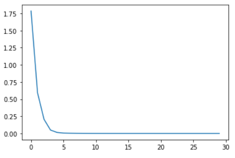
epoch : 5, tr_loss : 0.015
epoch : 10, tr_loss : 0.001
epoch : 15, tr_loss : 0.000
epoch : 20, tr_loss : 0.000
epoch : 25, tr_loss : 0.000
epoch : 30, tr_loss : 0.000
6) Checking performance
yhat = model.predict(x_data)
yhat = np.argmax(yhat, axis=-1) * x_data_mask

pprint(list(map(lambda row : [idx2pos.get(elm) for elm in row],yhat.astype(np.int32).tolist())), width = 120)
pprint(pos)
[['pronoun', 'verb', 'adjective', '<pad>', '<pad>', '<pad>', '<pad>', '<pad>', '<pad>', '<pad>'],
['noun', 'verb', 'adverb', 'adjective', '<pad>', '<pad>', '<pad>', '<pad>', '<pad>', '<pad>'],
['noun', 'verb', 'determiner', 'noun', 'preposition', 'adjective', 'noun', '<pad>', '<pad>', '<pad>'],
['noun', 'verb', 'adverb', 'adjective', 'verb', '<pad>', '<pad>', '<pad>', '<pad>', '<pad>']]
[['pronoun', 'verb', 'adjective'],
['noun', 'verb', 'adverb', 'adjective'],
['noun', 'verb', 'determiner', 'noun', 'preposition', 'adjective', 'noun'],
['noun', 'verb', 'adverb', 'adjective', 'verb']]
plt.plot(tr_loss_hist)
[<matplotlib.lines.Line2D at 0x23e9f137bc8>]
참고자료
https://www.edwith.org/boostcourse-dl-tensorflow/lecture/43754/
http://solarisailab.com/archives/1515