이번에 다룰 Many to one은 특히 자연어 처리 분야에서 어떤 문장, 또는 단어를 RNN으로 인코딩하고 해당 문장 또는 단어의 sentiment를 classification하는 데 활용할 수 있다.

먼저 간단하게 many to one의 활용 방법을 확인해보자. 예를 들어 'This movie is good'이라는 문장이 주어져 있을 때, 문장의 polarity를 파악하는 문제를 푼다고 가정해보자. 'This movie is good'문장을 단어의 시퀀스라고 생각해 문장을 ['This', 'movie', 'is', 'good']과 같이 단어 단위로 쪼갠 후 (이를 'Tokenization'라고 한다) Tokenization한 단어들을 RNN에 입력하면 RNN은 각각의 토큰을 읽고, 마지막 토큰을 읽었을 때 polarity를 분류하는 것이 바로 many to one방식이다.
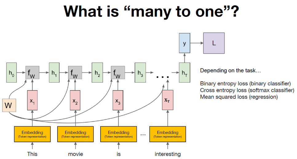
조금 더 자세히 작동원리를 살펴보자. 사실 RNN은 토큰인 단어 자체를 처리할 수 없다. 그러므로 토큰을 숫자vector로 바꿔주는 Embedding layer가 존재한다. 참고로 이 Embedding layer는 활용하는 방식에 따라 학습을 할 수도 있고 안 할 수도 있다. Embedding layer가 각각의 토큰을 RNN이 처리할 수 있도록 만들어주면, RNN은 토큰을 순서대로 읽어들이고 마지막 토큰을 읽었을 때 나온 출력과 정답간의 loss를 계산한다. 그리고 이 loss를 기반으로 back popagation하여 RNN을 학습한다.
이제 예제를 바탕으로 many to one RNN을 구현해보자.
1. Importing libraries
# setup
import numpy as np
import tensorflow as tf
import matplotlib.pyplot as plt
from tensorflow import keras
from tensorflow.keras import layers
from tensorflow.keras import Sequential, Model
from tensorflow.keras.preprocessing.sequence import pad_sequences
%matplotlib inline

print(tf.__version__)
2. Preparing data set
# example data
words = ['good', 'bad', 'worse', 'so good']
y_data = [1,0,0,1] # 긍정은 1 부정은 0의 레이블 값을 부여하였다.

# creating a token dictionary
# 예제 데이터로 주어진 각각의 단어를 캐릭터의 시퀀스로 간주하고 문제를 풀 것이다.
# 이를 위해서는 토큰인 캐릭터를 integer index로 맵핑하고 있는 토큰의 dictionary를 만들어야 한다.
# 여기서 character가 아닌 pad라는 토큰이 추가되는 이유는
# CNN, RNN을 막론하고 딥러닝에서는 batch단위의 연산이 효율적이므로
# 데이터가 서로 다른 시퀀스의 length를 가진 경우 길이를 맞춰줘야할 필요가 있기 때문이다.
char_set = ['<pad>'] + sorted(list(set(''.join(words))))
idx2char = {idx : char for idx, char in enumerate(char_set)}
char2idx = {char : idx for idx, char in enumerate(char_set)}

print(char_set)
print(idx2char)
print(char2idx)
['<pad>', ' ', 'a', 'b', 'd', 'e', 'g', 'o', 'r', 's', 'w']
{0: '<pad>', 1: ' ', 2: 'a', 3: 'b', 4: 'd', 5: 'e', 6: 'g', 7: 'o', 8: 'r', 9: 's', 10: 'w'}
▶ 출력을 해보면 각각의 토큰이 integer index와 맵핑이 돼있는 것을 확인할 수 있다.
{'<pad>': 0, ' ': 1, 'a': 2, 'b': 3, 'd': 4, 'e': 5, 'g': 6, 'o': 7, 'r': 8, 's': 9, 'w': 10}
# converting sequence of tokens to sequence of indices
# 생성한 toke dictionary를 기반으로 단어를 integer index의 시퀀스로 변환할 수 있다.
x_data = list(map(lambda word : [char2idx.get(char) for char in word], words))
x_data_len = list(map(lambda word : len(word), x_data))

print(x_data)
print(x_data_len)
[[6, 7, 7, 4], [3, 2, 4], [10, 7, 8, 9, 5], [9, 7, 1, 6, 7, 7, 4]]
▶ 출력을 해보면 각각의 단어가 integer index의 시퀀스로 변환된 것을 확인할 수 있다.
[4, 3, 5, 7]
# padding the sequence of indices
# 변환한 데이터를 pad_sequences function을 통해서 max_sequence가 가리키고 있는 값만큼의 길이로 padding을 해준다.
# 기본적으로 pad_sqeunces 함수는 0값으로 padding을 한다.
max_sequence = 10
x_data = pad_sequences(sequences = x_data, maxlen = max_sequence,
                       padding = 'post', truncating = 'post')

# checking data
print(x_data)
print(x_data_len)
print(y_data)
[[ 6 7 7 4 0 0 0 0 0 0] [ 3 2 4 0 0 0 0 0 0 0] [10 7 8 9 5 0 0 0 0 0] [ 9 7 1 6 7 7 4 0 0 0]]
[4, 3, 5, 7]
[1, 0, 0, 1]
3. Creating model
# creating simple rnn for "many to one" classification
input_dim = len(char2idx)
output_dim = len(char2idx)
one_hot = np.eye(len(char2idx))
hidden_size = 10
num_classes = 2

model = Sequential()
# layers.Embedding 메소드는 토큰을 one hot vector로 표현한다.
# one hot vector란 특정 토큰의 integer index 값에 해당하는 부분만 1이고 나머지는 0인 vector이다.
# 특히 mask_zero=True옵션을 통해 전처리 단계에서 0값으로 padding된 부분을 알아서 연산에서 제외할 수 있고,
# trainable=False옵션으로 one hot vector를 트레이닝하지 않을 수 있다.
model.add(layers.Embedding(input_dim=input_dim, output_dim=output_dim,
                           trainable=False, mask_zero=True, input_length=max_sequence,
                           embeddings_initializer=keras.initializers.Constant(one_hot)))
# layers.SimpleRNN은 기본적으로 시퀀스의 마지막 토큰을 인풋으로 받아 처리한 결과를 리턴한다.
model.add(layers.SimpleRNN(units=hidden_size))
# 이후 Dense를 이용하면 RNN을 many to one의 방식으로 활용하는 코드를 완성할 수 있다.
model.add(layers.Dense(units=num_classes))model.summary()Model: "sequential"
_________________________________________________________________
Layer (type) Output Shape Param #
=================================================================
embedding (Embedding) (None, 10, 11) 121
▶embedding layer에서 RNN이 데이터를 처리할 수 있도록 (data dimension, max sequence, input dimension)형태로 전처리했음을 확인할 수 있다.
_________________________________________________________________
simple_rnn (SimpleRNN) (None, 10) 220
▶ 이후 RNN에서는 설정한 hidden_size만큼의 벡터로 처리한다.
_________________________________________________________________
dense (Dense) (None, 2) 22
▶ 마지막으로 dense layer가 이를 classification한다.
=================================================================
Total params: 363 Trainable params: 242 Non-trainable params: 121
_________________________________________________________________
4. Training model
# 분류(classification)문제를 풀고 있기 때문에 오차함수로 cross entropy를 사용
def loss_fn(model, x, y):
    return tf.reduce_mean(tf.keras.losses.sparse_categorical_crossentropy(
        y_true=y, y_pred=model(x), from_logits=True))

# creating an optimizer
lr = .01
epochs = 30
batch_size = 2
opt = tf.keras.optimizers.Adam(learning_rate = lr) # tf.train.AdamOptimizer(2.1버전)
위의 코드에서 오차함수는 Tensorflow 2.0대의 버전이고 2.1대 버전의 코드를 작성하자면 아래와 같다.
def loss_fn(model, x, y):
return tf.losses.sparse_softmax_cross_entropy(labels = y , logits=model(x))
▶ 여기서 y의 데이터는 one hot vecotr의 형태가 아닌 integer형태이므로 이를 처리해줄 수 있는 tf.losses.sparse_softmax_cross_entropy함수를 사용
# generating data pipeline
tr_dataset = tf.data.Dataset.from_tensor_slices((x_data, y_data))
tr_dataset = tr_dataset.shuffle(buffer_size = 4)
tr_dataset = tr_dataset.batch(batch_size = batch_size)

print(tr_dataset)
<BatchDataset shapes: ((None, 10), (None,)), types: (tf.int32, tf.int32)>
# training
tr_loss_hist = []

for epoch in range(epochs):
    avg_tr_loss = 0
    tr_step = 0

    for x_mb, y_mb in tr_dataset:
        # with블록에서 mini_batch마다 cross_entropy loss를 계산하고
        with tf.GradientTape() as tape:
            tr_loss = loss_fn(model, x=x_mb, y=y_mb)
        # 기울기(gradient)를 계산
        grads = tape.gradient(target=tr_loss, sources=model.variables)
        opt.apply_gradients(grads_and_vars=zip(grads, model.variables))
        avg_tr_loss += tr_loss
        tr_step += 1
    else:
        avg_tr_loss /= tr_step
        tr_loss_hist.append(avg_tr_loss)

    if (epoch + 1) % 5 ==0:
        print('epoch : {:3}, tr_loss : {:.3f}'.format(epoch + 1, avg_tr_loss.numpy()))
epoch : 5, tr_loss : 0.187
epoch : 10, tr_loss : 0.036
epoch : 15, tr_loss : 0.012
epoch : 20, tr_loss : 0.006
epoch : 25, tr_loss : 0.004
epoch : 30, tr_loss : 0.003
5. Checking performance
yhat = model.predict(x_data)
yhat = np.argmax(yhat, axis=-1)
print('acc : {:.2%}'.format(np.mean(yhat == y_data)))
acc : 100.00%
plt.plot(tr_loss_hist)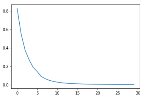
참고자료
https://www.edwith.org/boostcourse-dl-tensorflow/lecture/43751/
'IT > AI\ML' 카테고리의 다른 글
| [python/Tensorflow2.0] RNN(Recurrent Neural Network) ; many to many (0) | 2020.04.21 |
|---|---|
| [python/Tensorflow2.0] RNN(Recurrent Neural Network) ; many to one stacking (0) | 2020.04.21 |
| [python/Tensorflow2.0] RNN(Recurrent Neural Network) ; basic (0) | 2020.04.21 |
| [python/Tensorflow2.0] Mnist 학습 모델 (4)-CNN; Best CNN (0) | 2020.04.21 |
| [python/Tensorflow2.0] Mnist 학습 모델 (3)-CNN; Ensemble (0) | 2020.04.20 |