1) Numpy
- Numerical Python
- 파이썬의 고성능 과학 계산용 패키지
- Matrix와 Vector와 같은 Array 연산의 사실상의 표준
(1) Numpy의 특징
- 일반 List에 비해 빠르고, 메모리 효율적
- 반복문 없이 데이터 배열에 대한 처리를 지원
- 선형대수와 관련된 다양한 기능을 제공함
- C, C++, 포트란 등의 레거시 언어와 통합을 하여 개발이 가능함
(2) ndarray
- Numpy의 가장 기본이 되는 단위
(3) Array creation

import numpy as np

test_array = np.array(["1","4",5,8], float)
print(test_array)
type(test_array[3])

>> [1. 4. 5. 8.]
- numpy는 np.array함수를 활용하여 배열을 생성함 > ndarray
- numpy는 하나의 데이터 type만 배열에 넣을 수 있음
- List와 가장 큰 차이점, Dynaminc typing not supported
- C의 Array를 사용하여 배열을 생성함
test_array = np.array([1,4,5,"8"],float) #String Type의 데이터를 입력해도
print(test_array)
print(type(test_array[3])) # Float Type으로 자동 형변환 실시
print(test_array.dtype) #Array전체의 데이터 Type반환
print(test_array.shape) #Array의 shape(; vector, matrix, tesnsor의 크기, 형태 등에 대한 정보) 반환
[cf] Python List의 경우
Python List는 아래와 구조처럼되어 있으므로, 즉 메모리의 주소 위치만을 넣기 때문에, copy를 하더라도 메모리 주소가 복사된다.
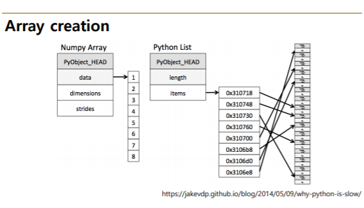
그러므로 deep copy를 위해서는 아래와 같이 코드를 작성한다.
import copy
copy.deepcopy(대상)
(4) Array Shape- ndim & size
- ndim : number of dimension
- size : 전체 데이터의 개수
tensor = [[[1,2,5,8], [1,2,5,8], [1,2,5,8]],
          [[1,2,5,8], [1,2,5,8], [1,2,5,8]],
          [[1,2,5,8], [1,2,5,8], [1,2,5,8]],
          [[1,2,5,8], [1,2,5,8], [1,2,5,8]]
        ]

np.array(tensor, int).ndim
>> 3

np.array(tensor, int).size
>> 48
(5) Array dtype
- Ndarray의 single element가 가지는 data type
- 각 element가 차지하는 memory의 크기가 결정됨
np.array([[1,2,3],[4.5,5,6]], dtype=int)
>> array([[1,2,3],
          [4,5,6]])
- C의 data type과 compatible
- nbytes : ndarray object의 메모리 크기를 반환
np.array([[1,2,3],[4.5, "5", "6"]],dtype=np.float32).nbytes
>>24
# 32bits = 4bytes => 6*4bytes
2) Data handling
(1) reshape
- Array의 shape 크기를 변경함 (element의 갯수는 동일)
import numpy as np

test_matrix = [[1,2,3,4], [1,2,5,8]]
x = np.array(test_matrix).shape
print(x)

>> (2, 4)

y = np.array(test_matrix).reshape(2,2,2)
print(y)

>> [[[1 2]
     [3 4]]

   [[1 2]
    [5 8]]]
reshape이 주로 사용되는 경우는 아래와 같다.
일반적으로 numpy의 출력 값은 vector형태이지만, 나중에 설명될 사이킷런에서는 matrix형태의 데이터를 사용해야하는데 이를 위해 reshape을 많이 이용한다.
- Array의 size만 같다면 다차원으로 자유롭게 변형 가능하다.
z = np.array(test_matrix).reshape(-1,2).reshape
# row의 개수를 정확하게 모르지만 column은 2개로 만들어 줄 때,
# 첫 번째 파라미터에 -1를 입력하면, size를 기반으로 row 개수를 선정하는 것(two dimensional array)이 가능하다.
print(z)
>> (4,2)
(2) flatten
- 다차원 array를 1차원 array로 변환
3) Indexing & slicing
(1) Indexing
- List와 달리 이차원 배열에서 [0, 0]과 같은 표기법을 제공함
- Matrix일 경우 앞은 row 뒤는 column을 의미함
import numpy as np
a = np.array([[1,2,3],[4.5,5,6]], int)
print(a)
print(a[0,0]) #Two dimensional array representation #1
print(a[0][0]) #Two dimensional array representation #2

a[0,0] = 12 # Matrix 0,0에 12할당
print(a)
a[0][0] = 5 # Matrix 0,0에 5할당
print(a)
(2) slicing

- List와 달리 행과 열 부분을 나눠서 slicing이 가능함
- Matrix의 부분 집합을 추출할 때 유용함
a = np.array([[1,2,3,4,5],[6,7,8,9,10]],int)
a[:,2:] # 전체 Row의 2열 이상
a[1,1:3] # 1Row의 1열 ~ 2열
a[1:3] # 1Row~2Row의 전체
4) Creation function
1) arange
- array의 범위를 지정하여, 값의 list를 생성하는 명령어
np.arange(30) # range : List의 range와 같은 효과, integer로 0부터 29까지 배열추출
>> [ 0  1  2  3  4  5  6  7  8  9 10 11 12 13 14 15 16 17 18 19 20 21 22 23
 24 25 26 27 28 29]
np.arange(0, 5, 0.5)
# 파라미터가 세 개일 경우 (시작, 끝, step)을 의미하며,
# step으로 floating point도 표시가능하다. (List의 경우는 불가능)
>> [0. 0.5 1. 1.5 2. 2.5 3. 3.5 4. 4.5]아까 배운 reshape도 같이 응용하여 사용할 수 있다.
np.arange(30).reshape(-1,5)
>> [[ 0  1  2  3  4]
 [ 5  6  7  8  9]
 [10 11 12 13 14]
 [15 16 17 18 19]
 [20 21 22 23 24]
 [25 26 27 28 29]]
2) ones, zeros and empty
zero : 0으로 가득찬 ndarray 생성
np.zeros(shape, dtype, order)np.zeros(shape=(10,), dtype=np.int8) # 10 - zero vector 생성
>> [0 0 0 0 0 0 0 0 0 0]np.zeros((2,5)) # 2 by 5 - zero matrix 생성
>> [[0. 0. 0. 0. 0.]
[0. 0. 0. 0. 0.]]
ones : 1로 가득찬 ndarray 생성, 사용법은 zeros와 동일
np.empty((2,5))
>> [[ 1.00441947e-311  1.00441948e-311 -8.99512849e+033  1.00441948e-311
   1.00441949e-311]
   [ 6.47283453e-253  1.00441944e-311  1.00441948e-311  4.20339843e-283
   1.00441946e-311]]
empty : shape만 주어지고 비어있는 ndarray 생성, 메모리 공간만 잡아주는 역할 (memory initialization이 되지 않음)
np.empty((2,5))
>> [[ 1.00441947e-311  1.00441948e-311 -8.99512849e+033  1.00441948e-311
   1.00441949e-311]
   [ 6.47283453e-253  1.00441944e-311  1.00441948e-311  4.20339843e-283
   1.00441946e-311]]
3) something_like
- 기존 ndarray의 shape 크기 만큼 1,0 또는 empty array를 반환
test_matrix = np.arange(30).reshape(5,6)
np.ones_like(test_matrix)
>> [[1 1 1 1 1 1]
 [1 1 1 1 1 1]
 [1 1 1 1 1 1]
 [1 1 1 1 1 1]
 [1 1 1 1 1 1]]
4) identity
- 단위 행렬(i 행렬)을 생성함
- 여기서 n은 number of rows
np.identity(n=3, dtype=np.int8)
>> [[1 0 0]
    [0 1 0]
    [0 0 1]]
5) eye
- 대각선인 1인 행렬, k로 시작 index의 변경(k = start index)이 가능
np.eye(N=3, M=5, dtype=np.int8)
>> [[1 0 0 0 0]
    [0 1 0 0 0]
    [0 0 1 0 0]]
np.eye(3, 5, k=2)
>> [[0. 0. 1. 0. 0.]
[0. 0. 0. 1. 0.]
[0. 0. 0. 0. 1.]]
6) diag
- 대각 행렬의 값을 추출한다. 여기서도 k는 start index이다.

matrix = np.arange(9).reshape(3,3)
np.diag(matrix)
>> [0 4 8]
matrix = np.arange(9).reshape(3,3)
np.diag(matrix, k=1)
>> [1 5]
7) random sampling
- 데이터 분포에 따른 sampling으로 array를 생성
np.random.uniform(0, 1, 10).reshape(2,5) #균등분포
>> [[0.26042239 0.70274925 0.93666132 0.25239196 0.57490808]
    [0.76052439 0.77588639 0.16689999 0.65610999 0.38467062]]
np.random.normal(0, 1, 10).reshape(2,5) #정규분포
>> [[ 1.73066902 0.67249815 0.53366579 1.85823518 -0.5619517 ]
[-0.50034208 -1.34827068 1.25100095 0.2986529 -0.95680724]]분포값을 이용하여 array를 만들 수 있다는 사실정도만 기억해도 괜찮다.
5) operation funtion
(1) sum
- ndarray의 element들 간의 합을 구함, list의 sum 기능과 동일
test_array = np.arange(1,11)
test_array.sum(dtype=np.float)
>> 55.0
(2) axis
- 모든 operation function을 실행할 때, 기준이 되는 dimension 축

- sum은 모든 요소를 더 하는 것이고, axis를 기준으로 연산
- axis가 늘어나면 새로 생기는 부분이 axis = 0 으로 갱신된다는 점을 주의

(3) mean & std
- ndarray의 element들 간의 평균 또는 표준편차를 반환
import numpy as np

test_array = np.arange(1,13).reshape(3,4)
x = test_array.mean()
y = test_array.mean(axis=0)
print (x, y)
>> 6.5 [5. 6. 7. 8.]
(4) Mathematical functions
- 그 외에도 다양한 수학 연산자를 제공함 (np.something 호출)
| exponential | trigonometric | hyperbolic |
| exp expm1 exp2 log log10 log1p log2 power sqrt |
sin cos tan acsin arccos atctan |
sinh cosh tanh acsinh arccosh arcranh |
(5) concatenate
- Numpy array를 합치는 함수

- vstack, hstack을 작성하지 않아도 앞에서 배운 axis를 기준으로 하여 합칠 수 있다.

- 참고로 데이터가 작으면 Numpy로 concatenate하는 것보다 Python의 List가 성능이 더 빠르다.
6) array operations
(1) Operations b/t arrays
- Numpy는 array간의 기본적인 사칙 연산을 지원한다.
test_a = np.array([1,2,3], [4,5,6], float)
test_a + test_a # Matrix + Matrix 연산
test_a - test_a # Matrix - Matrix 연산
test_a * test_a # Matrix내 element들 간의 같은 위치에 있는 값들끼리 연산
(2) Element-wise operations
- Array간 shape이 같을 때 일어나는 연산

(3) Dot product
- Matrix의 기본 연산
- dot 함수 사용

(4) transpose
- transpose 또는 T attribute 사용
import numpy as np

test_array = np.arange(1,7).reshape(2,3)
print(test_array)
>> [[1 2 3]
    [4 5 6]]

result = test_array.transpose() # 또는 test_array.T
print(result)
>> [[1 4]
    [2 5]
    [3 6]]
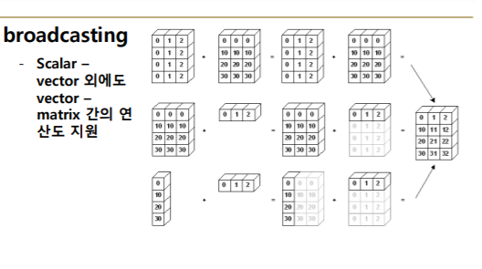
(5) broadcasting
- shape이 다른 배열 간 연산을 지원하는 기능

- Scalar-vector 이외에도 vector-matrix 간의 연산도 지원한다.
7) Numpy perfomance
- 일반적인 속도는 아래의 순서와 같다.
100,000,000번의 loop를 돌 때 약 4배 이상의 성능 차이를 보인다.
for loop < list comprehension < numpy
- Numpy는 C로 구현되어 있어, 성능을 확보하는 대신 파이썬의 가장 큰 특징인 dynamic typing을 포기함
- 대용량 계싼에서는 가장 흔히 사용됨
- 앞서 말했듯 Concatenate 처럼 계산이 아닌, 할당에서는 연산 속도의 이점이 없다.
8) comparisons
(1) All & Any
- Array의 데이터 전부(and) 또는 일부(or)가 조건에 만족 여부 반환
- any : 하나라도 저건에 만족한다면 true
- all : 모두가 조건에 만족해야 true
import numpy as np

a = np.arange(10)
result1, result2 = np.any(a>5), np.any(a<0)
print(result1, result2)
>> True False

result3, result4 =np.all(a>5), np.all(a<10)
print(result3, result4)
>> False True
(2) Comparsion operation
- Numpy는 배열의 크기가 동일 할 때 element간 비교의 결과를 Boolean type으로 반환하여 돌려줌
import numpy as np

test_a = np.array([1,3,0], float)
test_b = np.array([5,2,1], float)
print(test_a > test_b)
>>[False  True False]
a = np.array([1,3,0], float)
np.logical_and(a > 0, a < 3) # and 조건의 condition
>> [ True False False]import numpy as np
b = np.array([True, False, True], bool)
np.logical_not(b)
>> [False True False]import numpy as np
b = np.array([True, False, True], bool)
np.logical_not(b)
>> [False True False]
(3) np.where
np.where(condition, True, False)a = np.array([1,3,0], float)
np.where(a > 0, 3, 2)
>> [3 3 2]a = np.arange(10)
np.where(a>5) # Index값 반환
>> (array([6, 7, 8, 9], dtype=int64),)a = np.array([1, np.NaN, np.Inf], float)
np.isnan(a) # Not a number
>> [False True False]np.isfinite(a) # isfinite number
>> [ True False False]
(4) argmax & argmin
- array내 최대값 또는 최소값의 index를 반환함
a = np.array([1,2,4,5,8,78,23,3])
np.argmax(a), np.argmin(a)
>> 5, 0
- axis 기반의 반환
a = np.array([[1, 2, 4, 7],[9, 88, 6, 45], [9, 76, 3, 4]])
np.argmax(a, axis = 1), np.armin(a, axis=0)
>> [3 1 1] [0 0 2 2]
9) boolean & fancy index
추천기능 구현에 많이 사용된다.
(1) boolean index
- numpy는 주어진 배열을 특정 조건에 따른 값을 배열 형태로 추출 할 수 있다.
- Comparison operation 함수들도 모두 사용가능
import numpy as np

test_array = np.array([1, 4, 0, 2, 3, 8, 9, 7], float)
test_array > 3
>> [False  True False False False  True  True  True]
test_array[ test_array > 3 ] # 조건이 True인 index의 element만 추출
>> [4. 8. 9. 7.]condition = test_array < 3
test_array[condition]
>> [1. 0. 2.]
(2) fancy index
- numpy는 array를 index value로 사용해서 값을 추출하는 방법
import numpy as np

a =np.array([2, 4, 6, 8], float)
b = np.array([0, 0, 1, 3, 2, 1], int) #반드시 int형으로 선언
print(a[b]) # bracket index, b 배열의 값을 index로 하여 a의 값들을 추출함
>> [2. 2. 4. 8. 6. 4.]
print(a.take(b)) # take함수 : bracket index와 같은 효과 (위 방법보다 권장하는 방법)
>> [2. 2. 4. 8. 6. 4.]
- Matrix 형태의 데이터도 가능
import numpy as np

a = np.array([[1,4], [9,16]], float)
b = np.array([0, 0, 1, 1, 0], int)
c = np.array([0, 1, 1, 1, 1], int)
print(a[b,c]) # b를 row index, c를 column index로 변환하여 표시
>> [ 1.  4. 16. 16.  4.]
10) numpy data i/o
(1) loadtxt & savetxt
- Text type의 데이터를 읽고, 저장하는 기능
a = np.loadtxt("./population.txt")
a[:10] #파일 호출
a_int = a.astype(int)
a_int[:3] # Int type 변환np.savetxt('int_data.csv', a_int, delimiter=",") #int_data.csv로 저장
(2) numpy object - npy
- Numpy object(pickle)형태로 데이터를 저장하고 불러옴
- Binary 파일 형태로 저장함
np.save("npy_test", arr=a_int)npy_array = np.load(file= "npy_test.npy") # 말이 npy이지 python의 객체 저장방식인 pickle을 그대로 사용
npy_array[:3]참고자료
'IT > 언어' 카테고리의 다른 글
| [python] 머신러닝을 위한 Python(7) ; Data Handling - Pandas # 2 (0) | 2020.06.05 |
|---|---|
| [python] 머신러닝을 위한 Python(6); Data Handling - Pandas # 1 (0) | 2020.06.04 |
| [python] 머신러닝을 위한 Python(4) (0) | 2020.06.04 |
| [python] 머신러닝을 위한 Python(3) (0) | 2020.06.03 |
| [python] 머신러닝을 위한 Python(2) (0) | 2020.06.03 |